Stata 15 includes the ability to add transparency in graphs. What’s transparency you ask? Transparency is relevant when you have graphical elements that overlap. Without any transparency the element that is in front will completely obscure any elements behind it. Transparency solves that problem.
Suppose you want to plot two normal distributions. You can use the twoway function graph type to accomplish this (see Stata: Graphing Distributions). If the distributions overlap at all, it will be difficult to fully appreciate how much they overlap because the distribution in front will obscure the distribution in back. Here’s an example:
twoway function y = normalden(x), range(-4 4) ///
        color(eltgreen) recast(area) ///
    || function y = normalden(x+.5), range(-4 4) ///
        color(ebblue) recast(area) ///
        scheme(burd) legend(off)
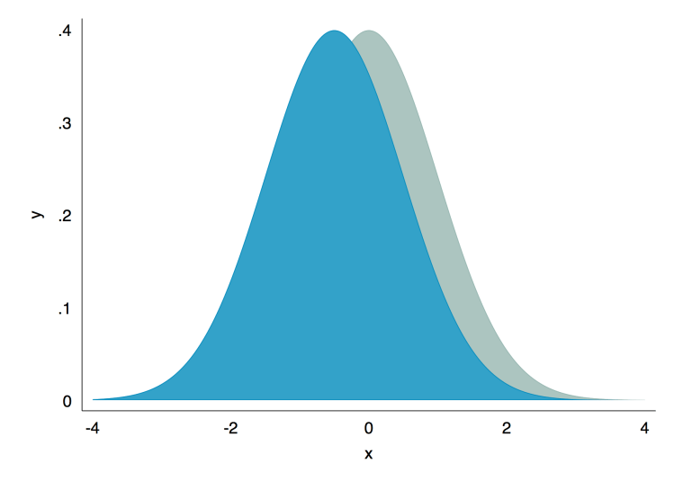
As you can see, the the blue distribution obscures the green. To fix this, we add transparency to the blue distribution. This is done by changing the color to color(ebblue%40). This makes the blue distribution 40% opaque.
twoway function y = normalden(x), range(-4 4) ///
        color(eltgreen) recast(area) ///
    || function y = normalden(x+.5), range(-4 4) ///
        color(ebblue%40) recast(area) ///
        scheme(burd) legend(off)
Trying fiddling around with the percentage to see how it affects things.
